Dremel made simple with Parquet
By @J_Wednesday, 11 September 2013 [
](https://blog.twitter.com/engineering/en_us/a/2013/dremel-made-simple-with-parquet.html#)[
](https://blog.twitter.com/engineering/en_us/a/2013/dremel-made-simple-with-parquet.html#)[
](https://blog.twitter.com/engineering/en_us/a/2013/dremel-made-simple-with-parquet.html#)[
](https://blog.twitter.com/engineering/en_us/a/2013/dremel-made-simple-with-parquet.html#)
Columnar storage is a popular technique to optimize analytical workloads in parallel RDBMs. The performance and compression benefits for storing and processing large amounts of data are well documented in academic literature as well as several commercial analytical databases.
The goal is to keep I/O to a minimum by reading from a disk only the data required for the query. Using Parquet at Twitter, we experienced a reduction in size by one third on our large datasets. Scan times were also reduced to a fraction of the original in the common case of needing only a subset of the columns. The principle is quite simple: instead of a traditional row layout, the data is written one column at a time. While turning rows into columns is straightforward given a flat schema, it is more challenging when dealing with nested data structures.
We recently introduced Parquet, an open source file format for Hadoop that provides columnar storage. Initially a joint effort between Twitter and Cloudera, it now has many other contributors including companies like Criteo. Parquet stores nested data structures in a flat columnar format using a technique outlined in the Dremel paper from Google. Having implemented this model based on the paper, we decided to provide a more accessible explanation. We will first describe the general model used to represent nested data structures. Then we will explain how this model can be represented as a flat list of columns. Finally we’ll discuss why this representation is effective.
To illustrate what columnar storage is all about, here is an example with three columns.
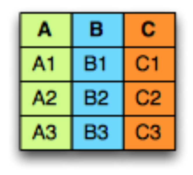
In a row-oriented storage, the data is laid out one row at a time as follows:

Whereas in a column-oriented storage, it is laid out one column at a time:

There are several advantages to columnar formats.
Organizing by column allows for better compression, as data is more homogenous. The space savings are very noticeable at the scale of a Hadoop cluster.
I/O will be reduced as we can efficiently scan only a subset of the columns while reading the data. Better compression also reduces the bandwidth required to read the input.
As we store data of the same type in each column, we can use encodings better suited to the modern processors’ pipeline by making instruction branching more predictable.
The model
To store in a columnar format we first need to describe the data structures using a schema. This is done using a model similar to Protocol buffers. This model is minimalistic in that it represents nesting using groups of fields and repetition using repeated fields. There is no need for any other complex types like Maps, List or Sets as they all can be mapped to a combination of repeated fields and groups.
The root of the schema is a group of fields called a message. Each field has three attributes: a repetition, a type and a name. The type of a field is either a group or a primitive type (e.g., int, float, boolean, string) and the repetition can be one of the three following cases:
required: exactly one occurrence
optional: 0 or 1 occurrence
repeated: 0 or more occurrences
For example, here’s a schema one might use for an address book:
message AddressBook {required string owner;repeated string ownerPhoneNumbers;repeated group contacts {required string name;optional string phoneNumber;}}
Lists (or Sets) can be represented by a repeating field.

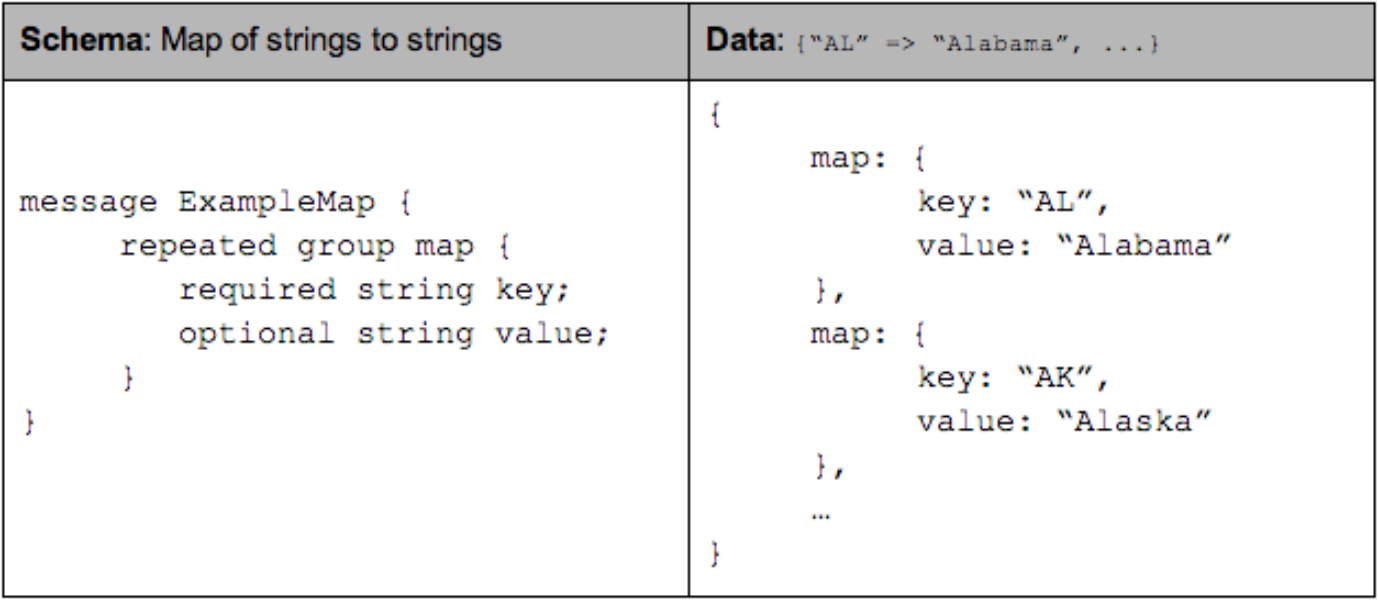
A Map is equivalent to a repeating field containing groups of key-value pairs where the key is required.
Columnar format
A columnar format provides more efficient encoding and decoding by storing together values of the same primitive type. To store nested data structures in columnar format, we need to map the schema to a list of columns in a way that we can write records to flat columns and read them back to their original nested data structure. In Parquet, we create one column per primitive type field in the schema. If we represent the schema as a tree, the primitive types are the leaves of this tree.
AddressBook example as a tree:
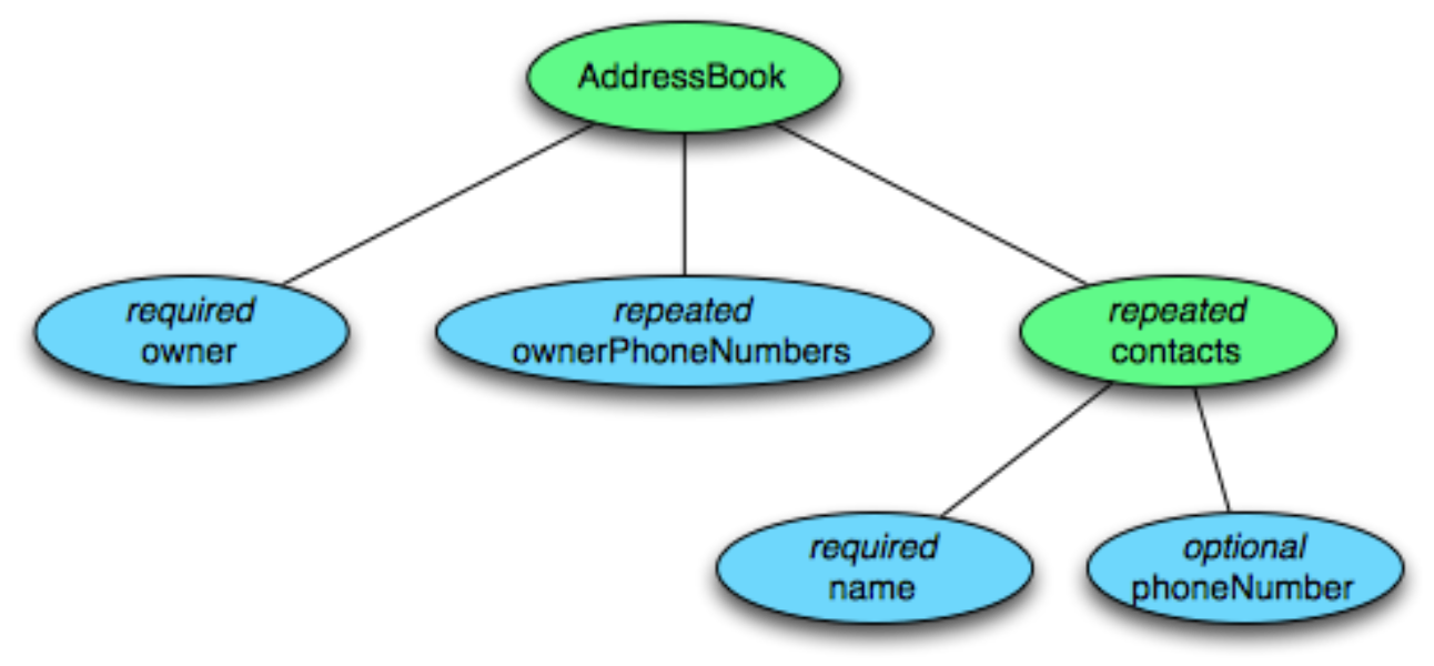
To represent the data in columnar format we create one column per primitive type cell shown in blue.

The structure of the record is captured for each value by two integers called repetition level and definition level. Using definition and repetition levels, we can fully reconstruct the nested structures. This will be explained in detail below.
Definition levels
To support nested records we need to store the level for which the field is null. This is what the definition level is for: from 0 at the root of the schema up to the maximum level for this column. When a field is defined then all its parents are defined too, but when it is null we need to record the level at which it started being null to be able to reconstruct the record.
In a flat schema, an optional field is encoded on a single bit using 0 for null and 1 for defined. In a nested schema, we use an additional value for each level of nesting (as shown in the example), finally if a field is required it does not need a definition level.
For example, consider the simple nested schema below:
message ExampleDefinitionLevel {optional group a {optional group b {optional string c;}}}
It contains one column: a.b.c where all fields are optional and can be null. When c is defined, then necessarily a and b are defined too, but when c is null, we need to save the level of the null value. There are 3 nested optional fields so the maximum definition level is 3.
Here is the definition level for each of the following cases:

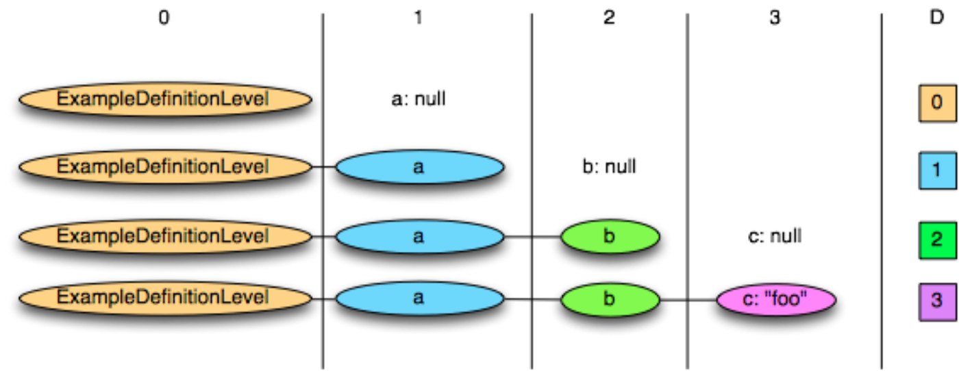
The maximum possible definition level is 3, which indicates that the value is defined. Values 0 to 2 indicate at which level the null field occurs.
A required field is always defined and does not need a definition level. Let’s reuse the same example with the field b now required:
message ExampleDefinitionLevel {optional group a {required group b {optional string c;}}}
The maximum definition level is now 2 as b does not need one. The value of the definition level for the fields below b changes as follows:
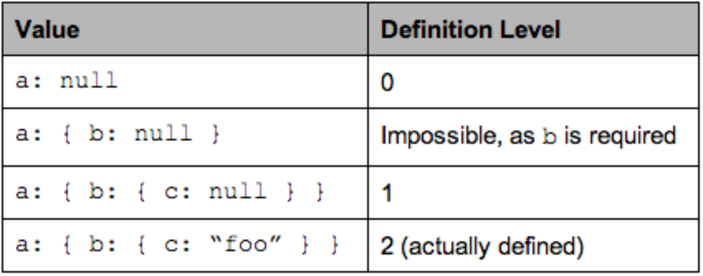
Making definition levels small is important as the goal is to store the levels in as few bits as possible.
Repetition levels
To support repeated fields we need to store when new lists are starting in a column of values. This is what repetition level is for: it is the level at which we have to create a new list for the current value. In other words, the repetition level can be seen as a marker of when to start a new list and at which level. For example consider the following representation of a list of lists of strings:
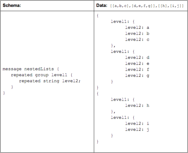
The column will contain the following repetition levels and values:
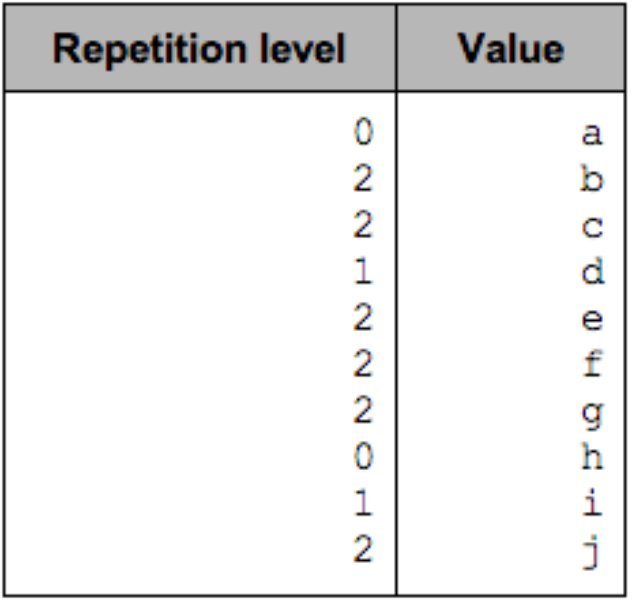
The repetition level marks the beginning of lists and can be interpreted as follows:
0 marks every new record and implies creating a new level1 and level2 list
1 marks every new level1 list and implies creating a new level2 list as well.
2 marks every new element in a level2 list.
On the following diagram we can visually see that it is the level of nesting at which we insert records:
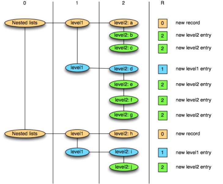
A repetition level of 0 marks the beginning of a new record. In a flat schema there is no repetition and the repetition level is always 0. Only levels that are repeated need a Repetition level: optional or required fields are never repeated and can be skipped while attributing repetition levels.
Striping and assembly
Now using the two notions together, let’s consider the AddressBook example again. This table shows the maximum repetition and definition levels for each column with explanations on why they are smaller than the depth of the column:

In particular for the column contacts.phoneNumber, a defined phone number will have the maximum definition level of 2, and a contact without phone number will have a definition level of 1. In the case where contacts are absent, it will be 0.
AddressBook {owner: "Julien Le Dem",ownerPhoneNumbers: "555 123 4567",ownerPhoneNumbers: "555 666 1337",contacts: {name: "Dmitriy Ryaboy",phoneNumber: "555 987 6543",},contacts: {name: "Chris Aniszczyk"}}AddressBook {owner: "A. Nonymous"}
We’ll now focus on the column contacts.phoneNumber to illustrate this.
Once projected the record has the following structure:
AddressBook {contacts: {phoneNumber: "555 987 6543"}contacts: {}}AddressBook {}
The data in the column will be as follows (R = Repetition Level, D = Definition Level)
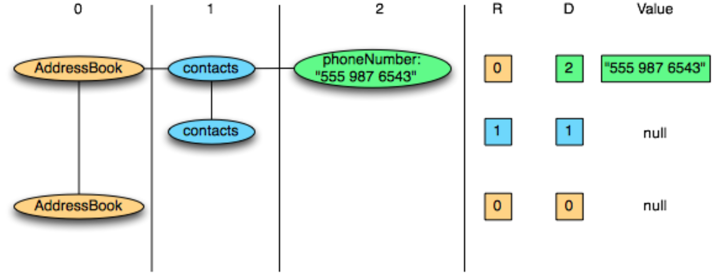
To write the column we iterate through the record data for this column:
contacts.phoneNumber: “555 987 6543”new record: R = 0
value is defined: D = maximum (2)
contacts.phoneNumber: nullrepeated contacts: R = 1
only defined up to contacts: D = 1
contacts: nullnew record: R = 0
only defined up to AddressBook: D = 0
The columns contains the following data:
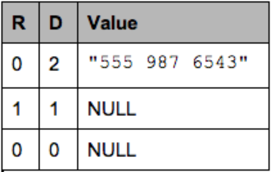
Note that NULL values are represented here for clarity but are not stored at all. A definition level strictly lower than the maximum (here 2) indicates a NULL value.
To reconstruct the records from the column, we iterate through the column:
R=0, D=2, Value = “555 987 6543”:R = 0 means a new record. We recreate the nested records from the root until the definition level (here 2)
D = 2 which is the maximum. The value is defined and is inserted.
R=1, D=1:R = 1 means a new entry in the contacts list at level 1.
D = 1 means contacts is defined but not phoneNumber, so we just create an empty contacts.
R=0, D=0:R = 0 means a new record. we create the nested records from the root until the definition level
D = 0 => contacts is actually null, so we only have an empty AddressBook
Storing definition levels and repetition levels efficiently
In regards to storage, this effectively boils down to creating three sub columns for each primitive type. However, the overhead for storing these sub columns is low thanks to the columnar representation. That’s because levels are bound by the depth of the schema and can be stored efficiently using only a few bits per value (A single bit stores levels up to 1, 2 bits store levels up to 3, 3 bits can store 7 levels of nesting). In the address book example above, the column owner has a depth of one and the column contacts.name has a depth of two. The levels will always have zero as a lower bound and the depth of the column as an upper bound. Even better, fields that are not repeated do not need a repetition level and required fields do not need a definition level, bringing down the upper bound.
In the special case of a flat schema with all fields required (equivalent of NOT NULL in SQL), the repetition levels and definition levels are omitted completely (they would always be zero) and we only store the values of the columns. This is effectively the same representation we would choose if we had to support only flat tables.
These characteristics make for a very compact representation of nesting that can be efficiently encoded using a combination of Run Length Encoding and bit packing. A sparse column with a lot of null values will compress to almost nothing, similarly an optional column which is actually always set will cost very little overhead to store millions of 1s. In practice, space occupied by levels is negligible. This representation is a generalization of how we would represent the simple case of a flat schema: writing all values of a column sequentially and using a bitfield for storing nulls when a field is optional.
Get Involved
Parquet is still a young project; to learn more about the project see our README or look for the “pick me up!” label on GitHub. We do our best to review pull requests in a timely manner and give thorough and constructive reviews.
You can also join our mailing list and tweet at @ApacheParquet to join the discussion.
